This vignette covers advanced irelink workflows for
readers who have already worked through the Getting Started or
Deduplication vignette. All examples use fake_1000 and a
shared in-memory DuckDB connection.
Setup
Train a complete model on fake_1000 that will be reused
across sections.
library(irelink)
#>
#> Attaching package: 'irelink'
#> The following object is masked from 'package:base':
#>
#>     months
library(ggplot2)

df <- fake_1000
con <- DBI::dbConnect(duckdb::duckdb())

spec <- il_spec() |>
  il_compare(first_name, cl_name()) |>
  il_compare(surname, cl_name()) |>
  il_compare(dob, cl_dob()) |>
  il_compare(city, cl_exact(term_frequency = TRUE)) |>
  il_compare(email, cl_email()) |>
  il_block_on(first_name) |>
  il_block_on(surname) |>
  il_block_on(city)

model <- il_model(df, spec = spec, con = con)
model <- il_estimate_prior(
  model,
  block_on(first_name, surname),
  block_on(email),
  recall = 0.6
)
model <- il_estimate_u(model, max_pairs = 1e5)
model <- il_estimate_em(model, block_on(first_name))
#> EM trained: surname, dob, city, and
#> email | skipped (blocked on): first_name
model <- il_estimate_em(model, block_on(dob))
#> EM trained: first_name, surname, city, and
#> email | skipped (blocked on): dob

pairs <- predict(model, threshold = 0.5)
clusters <- il_cluster(pairs, threshold = 0.85)
Training diagnostics
il_training_history() returns the m and u estimates from
each EM iteration across all training sessions. Plot it to check
convergence:
hist <- il_training_history(model)
autoplot(hist)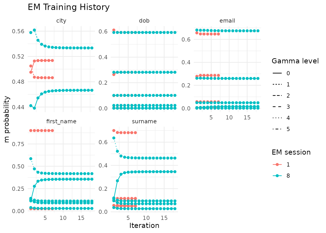
A well-converged model has stable values in the final iterations. If the estimates still drift, run more EM passes with different blocking rules or expand the candidate pairs.
Pair inspection
il_compare_records() scores a single pair of records
against the spec. Use it to see why a known match scores too low or a
non-match scores too high.
rec_a <- fake_1000[1, ]
rec_b <- fake_1000[5, ]

il_compare_records(rec_a, rec_b, spec = model$spec, con = con)
#> # A tibble: 1 × 5
#>   gamma_first_name gamma_surname gamma_dob gamma_city gamma_email
#>              <int>         <int>     <int>      <int>       <int>
#> 1                0            -1         1          0           0
The gamma columns show the comparison level reached on each field.
Use il_weights(model) to see the match-weight contribution
of each level.
Use a waterfall chart to see how field-level scores combine into one match decision:
autoplot(pairs, which = 1)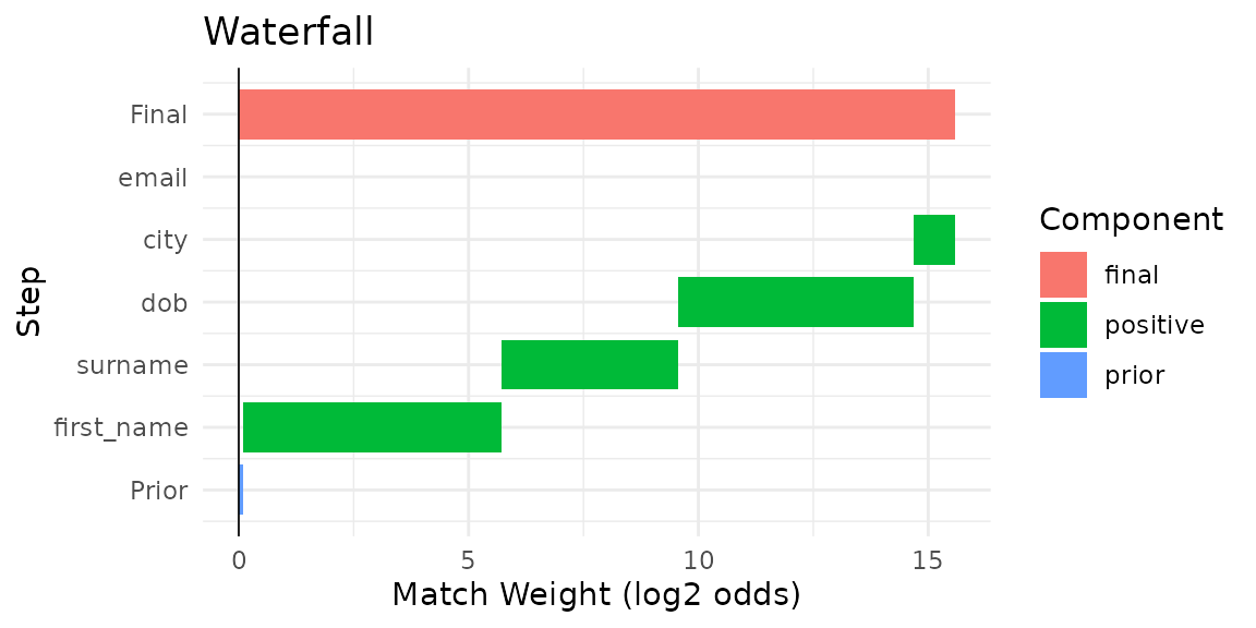
Lazy prediction for large data
predict(collect = FALSE) keeps scored pairs in the
database instead of collecting them into R. This path requires DuckDB or
PostgreSQL and is especially useful when materializing millions of rows
would exhaust memory. The examples here use DuckDB, and
il_cluster() detects the lazy reference so it can run
connected-components analysis in SQL.
pairs_lazy <- predict(model, threshold = 0.5, collect = FALSE)
pairs_lazy
#> <il_compared_lazy> 2,783 pairs in table __il_9011_1_predicted_4 (threshold = 0.5)
Pass the lazy reference directly to il_cluster():
clusters_lazy <- il_cluster(pairs_lazy, threshold = 0.85)
nrow(clusters_lazy)
#> [1] 952
autoplot() and il_waterfall() collect
automatically when needed, so downstream analysis code stays the same.
Use the lazy path on DuckDB or PostgreSQL when candidate-pair counts
exceed available memory. The lazy prediction table is model-scoped, and
il_cleanup(model) removes it along with the model’s source
and term-frequency tables.
Chunked u estimation and SQL profiling
For larger datasets, il_estimate_u() can accumulate
random-pair gamma counts in chunks and stop once every comparison level
has enough support:
model <- il_estimate_u(
  model,
  max_pairs = 5e6,
  chunk_size = 250000,
  min_count_per_level = 100
)
model$params$u_estimation
When you need to inspect database performance, set
profile_sql = TRUE on il_estimate_u(),
il_estimate_prior(), or predict() to collect
lightweight SQL timing metadata:
Cluster diagnostics
il_graph_metrics() computes node-level, edge-level, and
cluster-level summaries from the linkage graph. Use it to spot
thresholds that are too loose or clusters with unexpectedly low
density.
metrics <- il_graph_metrics(pairs, clusters)The cluster table reports size and internal edge density, which is the number of edges divided by the maximum possible number for a cluster of that size:
metrics$clusters
#> # A tibble: 142 × 5
#>    cluster_id  n_nodes n_edges density cluster_centralization
#>    <chr>         <int>   <int>   <dbl>                  <dbl>
#>  1 cluster_428       3       2   0.667                  1
#>  2 cluster_960       7      17   0.810                  0.267
#>  3 cluster_736       2       1   1                     NA
#>  4 cluster_879       5      14   1.4                    0.167
#>  5 cluster_911       7      21   1                      0
#>  6 cluster_296       5       9   0.9                    0.167
#>  7 cluster_907       4       4   0.667                  0.667
#>  8 cluster_149      16      61   0.508                  0.410
#>  9 cluster_301      10      41   0.911                  0.111
#> 10 cluster_814       7      23   1.10                   0.1
#> # ℹ 132 more rows
A large maximum cluster size with low density often means a
transitive link is pulling unrelated entities together. Consider raising
the threshold in predict() or il_cluster() and
then checking the metrics again.
The node table shows how many links each record participates in:
head(metrics$nodes)
#> # A tibble: 6 × 4
#>   unique_id cluster_id  degree node_centrality
#>   <chr>     <chr>        <int>           <dbl>
#> 1 164       cluster_164      8           1.14
#> 2 170       cluster_164      6           0.857
#> 3 166       cluster_164      8           1.14
#> 4 167       cluster_164      7           1
#> 5 169       cluster_164      6           0.857
#> 6 171       cluster_164      6           0.857
Records with unusually high degree relative to their cluster size may be acting as hubs that inflate the cluster beyond its true membership.
Phonetic blocking
Standard equality blocking misses pairs where names sound alike but
are spelled differently. Examples include “Smith” and “Smyth” or “Jon”
and “John”. Pass .transform = il_soundex to
il_block_on() or block_on() to group names by
phonetic code instead of exact spelling.
spec_phon <- il_spec() |>
  il_compare(first_name, cl_name()) |>
  il_compare(surname, cl_name()) |>
  il_compare(dob, cl_dob()) |>
  il_block_on(first_name, .transform = il_soundex) |>
  il_block_on(surname, .transform = il_soundex)
Use the same .transform argument when you specify a
blocking rule for an EM training pass:
model_phon <- il_model(df, spec = spec_phon, con = con)
model_phon <- il_estimate_u(model_phon, max_pairs = 1e5)
model_phon <- il_estimate_em(
  model_phon,
  block_on(first_name, .transform = il_soundex)
)
#> EM trained: surname and dob | skipped (blocked on):
#> first_name
Phonetic blocking usually improves recall, but it also increases the
number of candidate pairs. Use il_count_pairs() to check
that trade-off before you commit to a spec.
Column transforms
The transform argument in il_compare()
applies a function to both values before scoring. Use it to normalize
case or remove whitespace before a similarity comparison:
spec_tr <- il_spec() |>
  il_compare(first_name, cl_jaro_winkler(0.9, 0.7), transform = tolower) |>
  il_compare(surname, cl_jaro_winkler(0.9, 0.7), transform = tolower) |>
  il_compare(dob, cl_exact()) |>
  il_block_on(first_name) |>
  il_block_on(surname)

model_tr <- il_model(df, spec = spec_tr, con = con)
model_tr <- il_estimate_u(model_tr, max_pairs = 1e5)
model_tr <- il_estimate_em(model_tr, block_on(surname))
#> EM trained: first_name and dob | skipped (blocked on):
#> surnametolower, toupper, and trimws
are translated to SQL on DuckDB and PostgreSQL, so they run in the
database. Custom R functions only work on the R-side path. When you save
a model with il_save(), .rds stores the R
object as is, while .json writes Splink settings SQL so
loaded comparisons come back as SQL-backed levels. Anonymous functions
still produce a warning on save.
Incremental matching
il_find_matches() scores new records against data that
is already loaded into a trained model, using the same blocking rules
and comparison spec.
new_df <- data.frame(
  first_name = c('Jhon', 'Alice'),
  surname    = c('Smith', 'Jones'),
  dob        = c('1990-01-15', '1985-06-20'),
  city       = c('London', 'Manchester'),
  email      = c(NA, 'ajones@example.com')
)

matches <- il_find_matches(model, new_df, threshold = 0.5)
matches
#> # A tibble: 17 × 5
#>    unique_id_l unique_id_r match_weight total_match_weight match_probability
#>          <int>       <int>        <dbl>              <dbl>             <dbl>
#>  1           1         239        0.832              0.925             0.655
#>  2           1         364        0.832              0.925             0.655
#>  3           1         241        0.832              0.925             0.655
#>  4           1         362        2.28               2.37              0.838
#>  5           1         367        0.832              0.925             0.655
#>  6           1         238        2.31               2.41              0.841
#>  7           1         791        0.832              0.925             0.655
#>  8           1         240        0.832              0.925             0.655
#>  9           2         858        0.871              0.964             0.661
#> 10           1         363        0.832              0.925             0.655
#> 11           2         864        0.871              0.964             0.661
#> 12           2         859        2.31               2.41              0.841
#> 13           1         237        2.28               2.37              0.838
#> 14           1         365        0.832              0.925             0.655
#> 15           1         242        0.832              0.925             0.655
#> 16           1         366        0.832              0.925             0.655
#> 17           1         789        2.31               2.41              0.841
Each row is a (new record, existing record) pair.
unique_id_l identifies the new record (auto-assigned
starting from 1) and unique_id_r identifies the matched
record in the original dataset.
This works well with il_load() and
il_attach(). Load a saved model, attach it to the current
database, and call il_find_matches() for each incoming
batch of new records.
Cleanup
il_cleanup(model) only removes tables owned by that
model, so it is safe when several models share the same connection.
il_cleanup_all(con) is broader and is best reserved for
failed runs or exploratory sessions where you want to clear every
irelink table before disconnecting.
il_cleanup(model)
il_cleanup(model_phon)
il_cleanup(model_tr)
DBI::dbDisconnect(con, shutdown = TRUE)