This vignette walks through a full deduplication workflow on
fake_1000, covering model training, prediction, clustering,
and evaluation against ground-truth labels. The dataset comes from the
Python splink
library and contains 1,000 records for 181 unique people. Many records
include typos, missing values, and other realistic data-quality
issues.
Explore the data
df <- fake_1000
head(df)
#> # A tibble: 6 × 7
#>   unique_id first_name surname dob        city   email                   cluster
#>       <int> <chr>      <chr>   <chr>      <chr>  <chr>                     <int>
#> 1         0 Julia      NA      2015-10-29 London hannah88@powers.com           0
#> 2         1 Julia      Taylor  2015-07-31 London hannah88@powers.com           0
#> 3         2 Julia      Taylor  2016-01-27 London hannah88@powers.com           0
#> 4         3 Julia      Taylor  2015-10-29 NA     hannah88opowersc@m            0
#> 5         4 oNah       Watson  2008-03-23 Bolton matthew78@ballard-mcdo…       1
#> 6         5 Noah       Watson  2008-03-23 Bolton matthew78@ballard-mcdo…       1
The cluster column is the ground truth, so records that
share the same cluster value refer to the same person. There are 181
unique entities across 1000 records. Missing values appear as
NA, which reflects a common real-world problem.
Before building a model, profile the data to understand its completeness and value distributions:
con <- DBI::dbConnect(duckdb::duckdb())
comp <- il_completeness(df, con = con)
comp
#> # A tibble: 7 × 5
#>   table   column     n_total n_non_null pct_non_null
#>   <chr>   <chr>        <int>      <int>        <dbl>
#> 1 table_1 unique_id     1000       1000        100
#> 2 table_1 first_name    1000        900         90
#> 3 table_1 surname       1000        923         92.3
#> 4 table_1 dob           1000       1000        100
#> 5 table_1 city          1000        891         89.1
#> 6 table_1 email         1000        888         88.8
#> 7 table_1 cluster       1000       1000        100
autoplot(comp)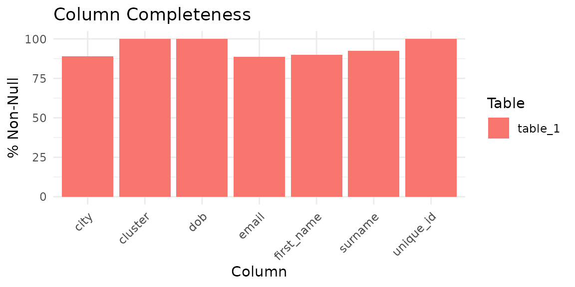
Check column value distributions to help choose blocking rules and comparisons:
il_profile(df[, c('first_name', 'surname', 'city')], con = con, top_n = 5)
#> # A tibble: 15 × 3
#>    column     value          n
#>    <chr>      <chr>      <dbl>
#>  1 first_name NA           100
#>  2 first_name George        22
#>  3 first_name Harry         18
#>  4 first_name Ivy           18
#>  5 first_name Noah          17
#>  6 surname    NA            77
#>  7 surname    Taylor        41
#>  8 surname    Jones         30
#>  9 surname    Brown         26
#> 10 surname    Thomas        18
#> 11 city       London       257
#> 12 city       NA           109
#> 13 city       Birmingham    36
#> 14 city       Leeds         33
#> 15 city       Sheffield     31
Choose blocking rules
il_suggest_blocking() lists candidate blocking columns
and ranks them. A good blocking key has high n_distinct,
which creates narrow blocks and fewer pairs, and high
coverage, which means fewer missing values:
il_suggest_blocking(df, con = con)
#> # A tibble: 6 × 6
#>   rule       n_distinct coverage n_pairs pct_of_cartesian score
#>   <chr>           <int>    <dbl>   <int>            <dbl> <dbl>
#> 1 dob               394    1        1850            0.370 0.996
#> 2 cluster           181    1        2975            0.596 0.994
#> 3 surname           317    0.923    3278            0.656 0.917
#> 4 first_name        326    0.9      2372            0.475 0.896
#> 5 email             336    0.888    1603            0.321 0.885
#> 6 city              174    0.891   36905            7.39  0.825
The spec below uses first_name, surname,
and city, which rank among the top columns here.
Define the specification
Choose the comparisons and blocking rules. Names use Jaro-Winkler
similarity, dates of birth use the cl_dob() helper, and
city uses exact matching with term-frequency adjustment:
spec <- il_spec() |>
  il_compare(first_name, cl_name()) |>
  il_compare(surname, cl_name()) |>
  il_compare(dob, cl_dob()) |>
  il_compare(city, cl_exact(term_frequency = TRUE)) |>
  il_compare(email, cl_email()) |>
  il_block_on(first_name) |>
  il_block_on(surname) |>
  il_block_on(city)

spec
#> Linkage Specification
#>   Comparisons (5):
#>     first_name : levels
#>     surname : levels
#>     dob : levels
#>     city : exact
#>     email : levels
#>   Blocking rules (3, OR-ed):
#>     1. first_name
#>     2. surname
#>     3. city
Estimate the number of pairs produced by each blocking rule:
il_count_pairs(
  df,
  block_on(first_name),
  block_on(surname),
  block_on(city),
  con = con
)
#> # A tibble: 3 × 4
#>   rule       n_pairs cumulative_pairs pct_of_cartesian
#>   <chr>        <dbl>            <dbl>            <dbl>
#> 1 first_name    2372             2372            0.475
#> 2 surname       3278             5042            1.01
#> 3 city         36905            40793            8.17
Train the model
model <- il_model(df, spec = spec, con = con)Estimate the prior match probability with deterministic rules:
model <- il_estimate_prior(
  model,
  block_on(first_name, surname),
  block_on(email),
  recall = 0.6
)
Estimate u-probabilities from random pairs and then estimate m-probabilities with EM:
model <- il_estimate_u(model, max_pairs = 1e5)
model <- il_estimate_em(model, block_on(first_name))
#> EM trained: surname, dob, city, and
#> email | skipped (blocked on): first_name
model <- il_estimate_em(model, block_on(dob))
#> EM trained: first_name, surname, city, and
#> email | skipped (blocked on): dob
Inspect the trained model
summary(model)
#> irelink Model
#>   Status: Trained
#>   Link type: dedupe
#>   Records: 1000
#>   Comparisons: 5
#>   Blocking rules: 3
#>
#>   Parameters:
#>     prior: 0.5161334
#>     comparisons: # A tibble: 23 × 4
#>      comparisons:    comparison gamma_level      m       u
#>      comparisons:    <chr>            <int>  <dbl>   <dbl>
#>      comparisons:  1 first_name           0 0.355  0.967
#>      comparisons:  2 first_name           1 0.110  0.0187
#>      comparisons:  3 first_name           2 0.0278 0.00213
#>      comparisons:  4 first_name           3 0.0894 0.00370
#>      comparisons:  5 first_name           4 0.417  0.00852
#>      comparisons:  6 surname              0 0.346  0.966
#>      comparisons:  7 surname              1 0.0941 0.0173
#>      comparisons:  8 surname              2 0.0274 0.00189
#>      comparisons:  9 surname              3 0.0696 0.00295
#>      comparisons: 10 surname              4 0.463  0.0114
#>      comparisons: # ℹ 13 more rows
#>     u_estimation: 1e+05
#>      u_estimation: FALSE
#>      u_estimation: NULL
#>      u_estimation: NULL
#>      u_estimation: 100000
#>      u_estimation: 1
The match weights chart shows how much each comparison separates matches from non-matches:
autoplot(model)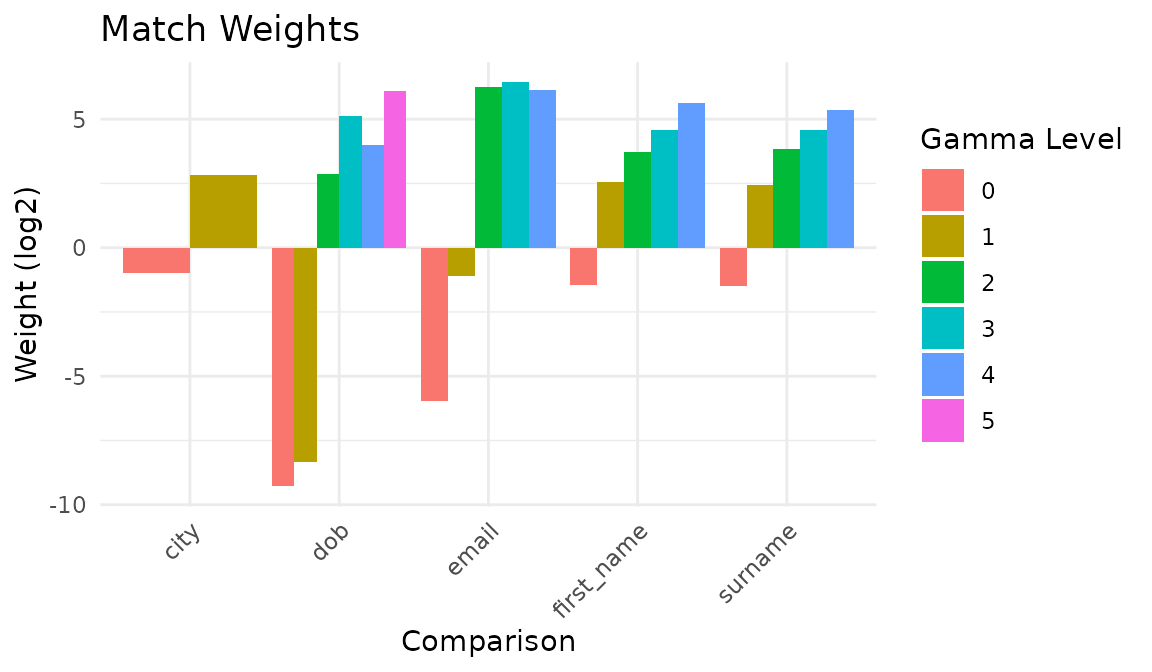
The parameter chart shows the raw m and u probabilities:
autoplot(model, type = 'parameters')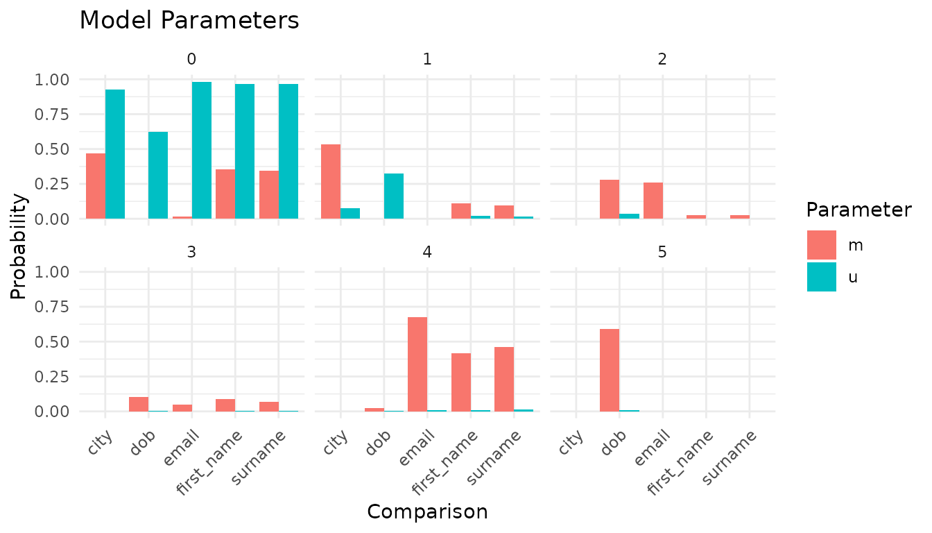
Save and reuse the model
Once you are satisfied with the parameters, save the model to disk. The saved file stores the spec and trained parameters so you can reuse the model without retraining:
Load the saved model with il_load() and attach it to the
same data or to new data with il_attach():
con2 <- DBI::dbConnect(duckdb::duckdb())
loaded <- il_load(path)
model2 <- il_attach(loaded, fake_1000, con = con2)
head(predict(model2, threshold = 0.85))
#> # A tibble: 6 × 11
#>   unique_id_l unique_id_r gamma_first_name gamma_surname gamma_dob gamma_city
#>         <int>       <int>            <int>         <int>     <int>      <int>
#> 1         509         512                4             2         3          1
#> 2         100         104                4            -1         5          0
#> 3         150         152                4             4         2          1
#> 4         252         254                4             4         5          0
#> 5         215         217                4             4         5          0
#> 6         814         820                4             4         5          1
#> # ℹ 5 more variables: gamma_email <int>, match_weight <dbl>, tf_adj_city <dbl>,
#> #   total_match_weight <dbl>, match_probability <dbl>
DBI::dbDisconnect(con2, shutdown = TRUE)
This pattern is common in production workflows. Train once on a representative sample, save the model, and reuse it as new data arrives.
Predict and cluster
Score all candidate pairs and apply a probability threshold:
View the match-weight distribution:
autoplot(predictions)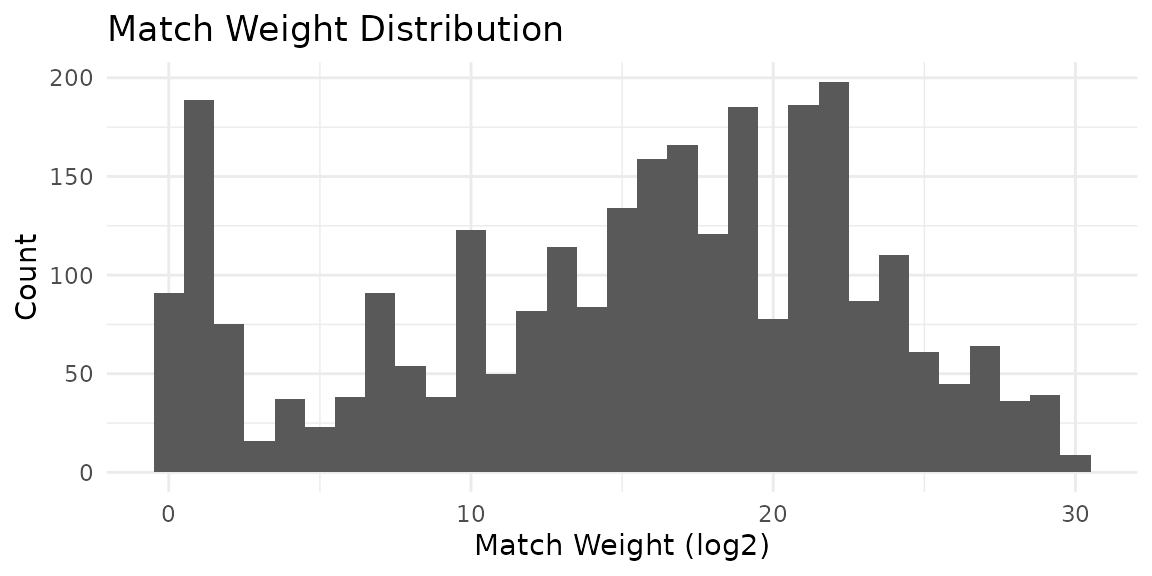
Use a waterfall chart to inspect how an individual pair is scored:
autoplot(predictions, which = 1)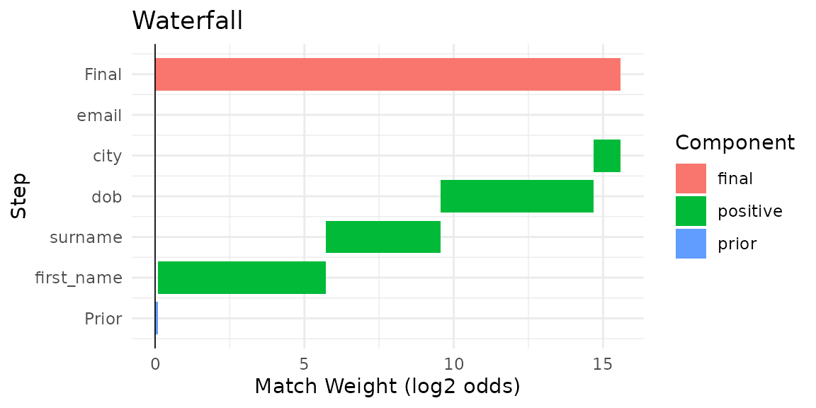
Resolve pairwise links into entity clusters:
clusters <- il_cluster(predictions, threshold = 0.85)
head(clusters)
#> # A tibble: 6 × 2
#>   unique_id cluster_id
#>   <chr>     <chr>
#> 1 628       cluster_626
#> 2 330       cluster_326
#> 3 793       cluster_792
#> 4 568       cluster_566
#> 5 599       cluster_599
#> 6 561       cluster_558
Evaluate against ground truth
The cluster column in the original data provides the
ground-truth entity labels. Convert them to pairwise labels for
evaluation:
# Use the bundled clerical labels from splink
labels_raw <- fake_1000_labels

# Rename to match irelink's evaluation convention
labels <- data.frame(
  unique_id_l = labels_raw$unique_id_l,
  unique_id_r = labels_raw$unique_id_r,
  is_match = as.integer(labels_raw$clerical_match_score)
)

nrow(labels)
#> [1] 3176
sum(labels$is_match)
#> [1] 2031
Accuracy metrics
acc <- il_accuracy(model, labels = labels)
acc
#> # A tibble: 419 × 16
#>     threshold    tp    fp    fn    tn fn_blocking_miss precision recall    f1
#>         <dbl> <int> <int> <int> <int>            <int>     <dbl>  <dbl> <dbl>
#>  1 0           1135   229   896   916              896     0.832  0.559 0.669
#>  2 0.00000183  1135   229   896   916              896     0.832  0.559 0.669
#>  3 0.00000353  1135   229   896   916              896     0.832  0.559 0.669
#>  4 0.00000498  1135   229   896   916              896     0.832  0.559 0.669
#>  5 0.00000512  1135   229   896   916              896     0.832  0.559 0.669
#>  6 0.00000960  1135   229   896   916              896     0.832  0.559 0.669
#>  7 0.00000986  1135   229   896   916              896     0.832  0.559 0.669
#>  8 0.0000139   1135   229   896   916              896     0.832  0.559 0.669
#>  9 0.0000255   1135   229   896   916              896     0.832  0.559 0.669
#> 10 0.0000268   1115   152   916   993              896     0.880  0.549 0.676
#> # ℹ 409 more rows
#> # ℹ 7 more variables: f2 <dbl>, f0_5 <dbl>, specificity <dbl>, npv <dbl>,
#> #   accuracy <dbl>, p4 <dbl>, phi <dbl>
autoplot(acc)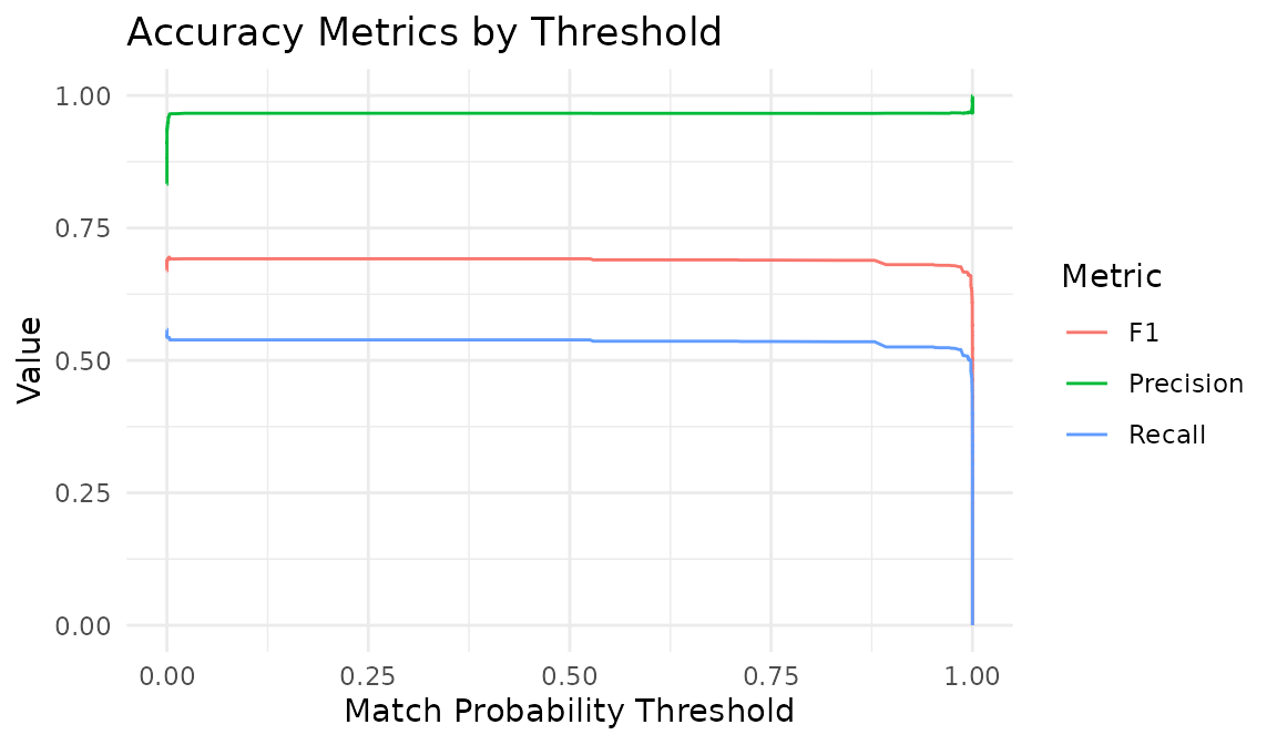
Error inspection
Examine false positives and false negatives at a specific threshold:
errors <- il_errors(model, labels = labels, threshold = 0.85)
head(errors)
#> # A tibble: 6 × 6
#>   unique_id_l unique_id_r match_weight match_probability true_label error_type
#>         <int>       <int>        <dbl>             <dbl> <lgl>      <chr>
#> 1           4           7        17.1              1.000 FALSE      false_posit…
#> 2           4           8         8.89             0.998 FALSE      false_posit…
#> 3           4           9        14.7              1.000 FALSE      false_posit…
#> 4           4          10        12.2              1.000 FALSE      false_posit…
#> 5           5           7        19.0              1.000 FALSE      false_posit…
#> 6           5           8         8.89             0.998 FALSE      false_posit…
Unlinkables
How many records remain unlinkable at each threshold?
unlink <- il_unlinkables(model)
autoplot(unlink)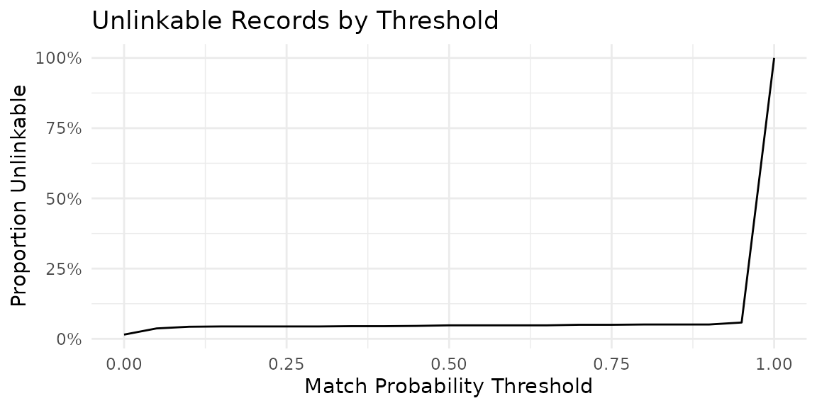
Cleanup
il_cleanup(model)
DBI::dbDisconnect(con, shutdown = TRUE)
il_cleanup(model) only removes tables owned by that
model. If an interactive run fails before you keep the model object,
call il_cleanup_all(con) to remove all irelink
tables from the connection before disconnecting.